Blogs

C Programming:

Theory Of Computation:

Finite State Machines: Definition: Capture patterns in behavior based on (limited) knowledge of what has happened in the past, and current input.

Introduction to Data Science

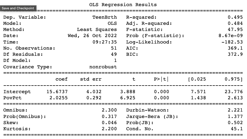
Code:
model = smf.ols (formula = 'TeenBrth ~ PovPct', data = df)
results = model.fit()
print(results.summary)

Output Table

Definitions:
1) coef : 𝛽1 estimate explaining the effect size
2) std err : standard error
3) P>|t| : the p-value
4) The 95% confidence interval: the 2.5 percentile on slope is under 2.5 and the 97.5% percentile is over 97.5.
- Says that you are 95% sure that it is within this range, so once it touches the zero slope line
- then there is a 5% chance that this is actually a null zero slope, they are related to eachother
- this is a model fit.

Q1: What is the effect size of the relationship between Poverty Percentage and Teen Birth Rate?
Answer: 2.03
Q2: Which value represents the expected Teen Birth Rate if the Poverty Percentage were 0?
Answer: 15.67: no matter what your poverty does, in the end there is always going to be a non-zero teen birth rate

Q3: What is our conclusion from this analysis? (Question: Does Poverty Percentage affect Teen Birth Rate?)
Answer: B) Reject the null; There is a relationship between Poverty Percentage and Teen Birth Rate
The numbers in the bottom section tells you how good is this fit.
The top section tells you statistics, what is this fit about, how much of the variance is being explained by the relationship.
The numbers is the middle are giving you the information on whether or not it a good fit.
Use statsmodels, use a linear model plot to quickly look at data, does the same general process as statsmodels but it is way less customizable (1 input for 1 output) 2) Linear model plot will not give you the coefficients out, it will not print them, it will return them to you, you can visually inspect them but you cannot know what those coefficients are. This is a design decision of seaborn. Visualization is for visualization, if you want to know what those coefficients, you have to use statsmodels.

Multiple Linear Regression: allows you to measure the effect of multiple predictors on an outcome.
Code:
mod = smf.ols(formula='TeenBrth ~ PovPct + ViolCrime', data=df)
res = mod.fit()
print(res.summary())

Setup and Data Wrangling

1. Import seaborn and apply its plotting styles
import seaborn as sns
sns.set(font_scale=2, style="white")

2. # import matplotlib
import matplotlib as mpl
import matplotlib.pyplot as plt
import matplotlib.style as style
# set plotting size parameter
plt.rcParams['figure.figsize'] = (17, 7)

3. # import pandas & numpy library
import pandas as pd
import numpy as np

4. # Statmodels & patsy
import patsy
import statsmodels.api as sm

To Convert Values of a Column to a Different Type
pulitzer['Daily Circulation, 2004'] = pulitzer['Daily Circulation, 2004'].str.replace(',','').astype(float)
pulitzer['Daily Circulation, 2013'] = pulitzer['Daily Circulation, 2013'].str.replace(',','').astype(float)
pulitzer['Change in Daily Circulation, 2004-2013'] = pulitzer['Change in Daily Circulation, 2004-2013'].str.replace('%','').astype(float)

To Display what type of values data are:
pultizer.dtypes

EDA and Visualization

Links

Matplotlib Colors Seaborn.distplot Documentation

Looking at Descriptive Stats of a Dataframe:
pultizer.describe()

Creating a plot that will help you see the differences and similarities of 2 columns of data: Histogram
fig, (ax1, ax2) = plt.subplots(ncols = 2, sharey = True)
sns.histplot(pulitzer['Daily Circulation, 2004'], bins = 40, ax = ax1, color = 'dimgrey')
sns.histplot(pulitzer['Daily Circulation, 2013'], bins = 40, ax = ax2, color = 'dimgrey')

Code to Find an Outlier
pulitzer[pulitzer['Change in Daily Circulation, 2004-2013'] == pulitzer['Change in Daily Circulation, 2004-2013'].max()]
KDE plots the Kernal Density Estimate

Inferential Analysis

Q: Relationship between the total number of Pulitzers and change in readership?

Tokenization

Before looking through data, you should check the following: duplicate responses, identification names, missingess, does it reflect reality, etc.
To get information about the size of the dataframe, use the .shape() method
Missing is how many no responses there are: use the .isnull() method which checks to see if there are empty values
String Method Documentation

Stop Words

Lexicon Normalization (Stemming)

In language, many different words come from the same root word. For example, "intersection", "intersecting", "intersects", and "intersected" are all related to the common root word, "intersect".
Stemming is how linguistic normalization occurs - it reduces words to their root words (and chops off additional things like 'ing') - all of the above words would be reduced to their common stem "intersect"
# Stemming
from ntlk.stem import PorterStemmer ps = PorterStemmer() stemmed_words = [] for w in filtered_sent: stemmed_words.append(ps.stem(w)) print("Filtered Sentence:", filtered_sent) print("Stemmed Sentence:", stemmed_words) Output:

Frequency Distribution

Which words are most frequently seen in a dataset?
# get series of all most and least liked words after stemming
# note that "No Response" is still being included in the analysis
most = df['most_stem'].apply(pd.Series).stack()
least = df['least_stem'].apply(pd.Series).stack()
FreqDist calculates the frequency of each word in the text and we can plot the most frequent words.

Text Analysis

Importing a dataset from a corpus.
Example: from nltk.corpus import inaugural
Example: inaugural.fieldids() (method that displays all of the txt files in the dataset)
Example: years = [fileid[:4] for fileid in inaugural.fileids()] getting the years from the txt file name.
Example: inaugural.raw('1793-Washington.txt') Choosing the contents of a single txt file.
Choose the dataframe, then the 'raw' method and then the txt file that you want the contents for.